Should I use Chapel or Julia for my next project?

Julia and Chapel are both newish languages aimed at productitive scientific computing, with parallel computing capabilities baked in from the start. There’s lots of information about both online, but not much comparing the two. If you are starting a new scientific computing project and are willing to try something new, which should you choose? What are their strengths and weaknesses, and how do they compare?

Here we walk through a comparison, focusing on distributed-memory parallelism of the sort one would want for HPC-style simulation. Both have strengths in largely disjoint areas. If you want matlib-like interactivity and plotting, and need only coodinator-worker parallelism, Julia is the clear winner; if you want MPI+OpenMPI type scability on rectangular distributed arrays (dense or sparse), Chapel wins handily. Both languages and environments have clear untapped potential and room to grow; we’ll talk about future prospects of the two languages at the end.

Update: I’ve updated the timings - I hadn’t been using @inbounds in the Julia code, and I had misconfigured my Chapel install so that the compiles weren’t optimized; this makes a huge difference on the 2d advection problem. All timings now are on an AWS c4.8x instance.

• A quick overview of the two languages
  • Julia
  • Chapel
• Similarities and differences
  • Standard library
  • Other packages
  • Language features
• Simple computational tasks
  • Linear algebra
  • Stencil calculation
  • Kmer counting
• Parallel primitives
  • Remote function execution
  • Futures, atomics and synchronization
  • Parallel loops, reductions, and maps
  • Threading
  • Distributed data
  • Communications
• A 2d advection problem
• Strengths, Weaknesses, and Future Prospects
  • Julia
  • Chapel
• My conclusions
  • Both projects are strong and useable, right now, at different things
  • Both projects have as-yet untapped potential

A quick overview of the two languages

Julia

The Julia project describes Julia as “a high-level, high-performance dynamic programming language for numerical computing.” It exploits type inference of rich types, just-in-time compilation, and multiple dispatch (think of R, with say print() defined to operate differently on scalars, data frames, or linear regression fits) to provide a dynamic, interactive, “scripting language”-type high level numerical programming language that gives performance less than but competitive with C or Fortran.

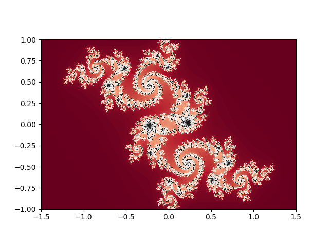
The project sees the language as more or less a matlab-killer, and so focusses on that sort of interface; interactive, through a REPL or Jupyter notebook (both available to try online), with integrated plotting; also, indexing begins at one, as God intended.¹

Example from David Sanders’ SciPy 2014 tutorial
using PyPlot # julia set function julia(z, c; maxiter=200) for n = 1:maxiter if abs2(z) > 4 return n-1 end z = z*z + c end return maxiter end jset = [ UInt8(julia(complex(r,i), complex(-.06,.67))) for i=1:-.002:-1, r=-1.5:.002:1.5 ]; get_cmap("RdGy") imshow(jset, cmap="RdGy", extent=[-1.5,1.5,-1,1])

Julia blurs the distinction between scientific users of Julia and developers in two quite powerful ways. The first is lisp-like metaprogramming, where julia code can be generated or modified from within Julia, making it possible to build domain-specific langauges (DSLs) inside Julia for problems; this allows simple APIs for broad problem sets which nonetheless take full advantage of the structure of the particular problems being solved; JuliaStats, DifferentialEquations.jl, JuliaFEM, and JuMP offer hints of what that could look like. Another sort of functionality this enables is Parallel Accellerator, an intel package that can rewrite some regular array operations into fast, vectorized native code. This code-is-data aspect of Julia, combined with the fact that much of Julia itself is written in Julia, puts user-written code on an equal footing with much “official” julia code.

The second way Julia blurs the line between user and developer is the package system which uses git and GitHub; this means that once you’ve installed someone’s package, you’re very close to being able to file a pull request if you find a bug, or to fork the package to specialize it to your own needs; and it’s similarly very easy to contribute a package if you’re already using GitHub to develop the package.

Julia has support for remote function execution (“out of the box” using SSH + TCP/IP, but other transports are available through packages), and distributed rectangular arrays; thread support is still experimental, as is shared-memory on-node arrays.

Chapel

While Julia is a scientific programming language with parallel computing support, Chapel is a programming language for parallel scientific computing. It is a PGAS language, with partitioned but globally-accessible variables, using GASNet for communications. It takes PGAS two steps further however than languages like Coarray Fortran, UPC, or X10.

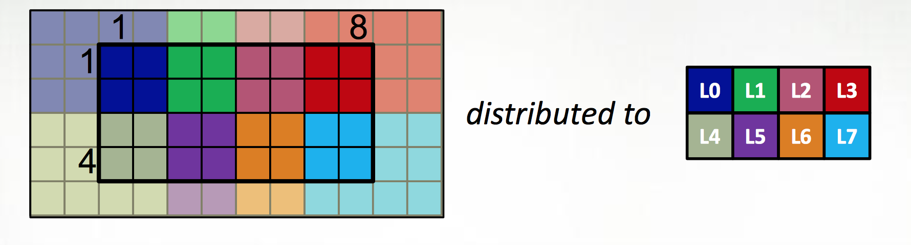
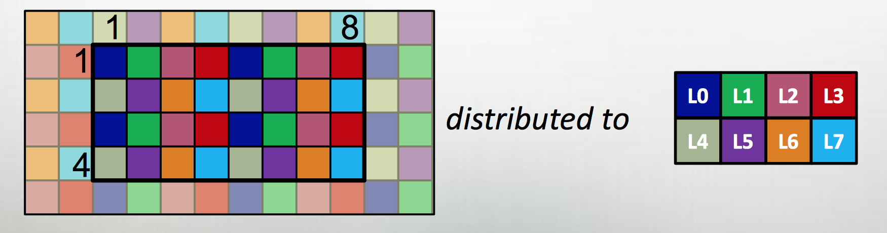
The first extension is to define all large data structures (arrays, associative arrays, graphs) as being defined over domains, and then definining a library of domain maps for distributing these domains over different locality regions (“locales”) (nodes, or NUMA nodes, or KNL accellerators) and layouts for describing their layout within a locale. By far the best tested and optimized domain maps are for the cases of dense (and to a lesser extent, CSR-layout sparse) rectangular arrays, as below, although there support for associative arrays (dictionaries) and unstructured meshes/graphs as well.

The second is to couple those domain maps with parallel iterators over the domains, meaning that one can loop over the data in parallel in one loop (think OpenMP) with a “global view” rather than expressing the parallelism explicitly as a SIMD-type program. This decouples the expression of the layout of the data from the expression of the calculation over the data, which is essential for productive parallel computing; it means that tweaking the layouts (or the dimensionality of the program, or…) doesn’t require rewriting the internals of the computation.

The distributions and layouts are written in Chapel, so that users can contribute new domain maps to the project.

Example from Chapel tutorial at ACCU 2017

var Dom: {1..4, 1..8} dmapped Block({1..4, 1..8});

var Dom: {1..4, 1..8} dmapped Cyclic(startIdx=(1,1));

// either case: var Inner : subdomain(Dom) = {2..3, 2..7}; const north = (-1,0), south = (1,0), east = (0,1), west = (0,-1); var data, data_new : [Dom] real; var delta : real; forall ij in Inner { data_new(ij) = (data(ij+north) + data(ij+south) + data(ij+east) + data(ij+west)) / 4.0; } delta = max reduce abs(data_new[Dom] - data[Dom]);

Chapel also exposes its lower-level parallel computing functionality — such as remote function execution, fork/join task parallelism — so that one can write a MPI-like SIMD program by explicity launching a function on each core:

coforall loc in Locales do 
    on loc do
        coforall tid in 0..#here.maxTaskPar do
            do_simd_program(loc, tid);

At roughly eight years old as a publically available project, Chapel is a slightly older and more mature language than Julia. However, the language continues to evolve and there are breaking changes between versions; these are much smaller and more localized breaking changes than with Julia, so that most recent example code online works readily. As its focus has always been on large-scale parallelism rather than desktop computing, its potential market is smaller so has attracted less interest and fewer users than Julia — however, if you read this blog, Chapel’s niche is one you are almost certainly very interested in. The relative paucity of users is reflected in the smaller number of contributed packages, although an upcoming package manager will likely lower the bar to future contributions.

Chapel also lacks a REPL, which makes experimentation and testing somewhat harder — there’s no equivalent of JuliaBox where one can play with the language at a console or in a notebook. There is an effort in that direction now which may be made easier by ongoing work on the underlying compiler architecture.

Similarities and differences

Standard library

Both Julia and Chapel have good documentation, and the basic modules or capabilities one would expect from languages aimed at technical computing:

• Complex numbers
• Mathematical function libraries
• Random numbers
• Linear algebra
• FFTs
• C, Python interoperability
• Multi-precision floats / BigInts
• MPI interoperability
• Profiling

although there are differences - in Julia, Python interoperability is much more complete (the Julia set example above used matplotlib plotting, while pychapel focuses on calling Chapel from within python). Also, Julia’s linear algebra support is much slicker, styled after Matlab syntax and with a rich set of matrix types (symmetric, tridiagonal, etc.), so that for linear solves, say, a sensible method is chosen automatically; the consise syntax and “do the right thing” approach are particularly helpful for interactive use², which is a primary use-case of Julia.

On profiling, the Julia support is primariy for serial profiling and text based; Chapel has a very nice tool called chplvis for visualizing parallel performance.

Other packages

Julia’s early adoption of a package management framework and very large initial userbase has lead to a very large ecosystem of contributed packages. As with all such package ecosystems, the packages themselves are a bit of a mixed bag – lots are broken or abandoned, many are simply wrappers to other tools – but there are also excellent, substantial packages taking full advantage of Julia’s capabalities that are of immediate interest to those doing scientific computing, such as DifferentialEquations.jl for ODEs, SDEs, and and FEM for some PDEs, BioJulia for bioinformatics, JuliaDiff for automatic differentiation, and JuliaStats for R-like statistical computing. The julia project would benefit from having a more curated view of the package listings easily available so that these high-quality tools were more readily visible to new users.

On the other hand, there are almost no packages available for Chapel outside of the main project. There are efforts to develop a package manager inspired by cargo (Rust) and glide (Go); this would be an important and needed development, almost certainly necessary to grow the Chapel community.

Language features

The biggest language feature difference is undoubtedly Julia’s JIT-powered lisp-metaprogramming capabilities; Chapel is a more statically-compiled language, with generics and reflection but not full lisp-like code-is-data. A small downside of Julia’s JIT approach is that functions are often slow the first time they are called, as they must be compiled. Relatedly, Julia is garbage-collected, which can lead to pauses and memory pressure at unexpected times. On the other hand, Chapel’s compile time, which is still quite long even compared to other compilers, makes the development cycle much slower than it would be with Julia or Python.

Beyond that, Julia and Chapel are both quite new and have functionality one might expect in a modern language: first class functions, lambda functions, comprehensions, keyword/optional parameters, type inference, generics, reflection, iterators, ranges, coroutines and green threads, futures, and JuliaDoc/chpldoc python packages for generating online documentation from source code and embedded comments.

More minor but something that quickly comes up: there’s difference in command-line argument handling which reflects the use cases each team finds important. Both give access to an argv-like array of strings passed to the command line; in base Julia with its interactive nature, that’s it (although there’s a nice python-argparse inspired contributed package), while in Chapel, intended to make compiled long-running executables one can define a constant (const n = 10;) and make it settable on the command line by prefixing the const with config and running the program with --n 20.

Simple computational tasks

Here we take a look at a couple common single-node scientific computation primitives in each framework (with Python for comparison) to compare the language features. Full code for the examples are available on GitHub.

Linear algebra

For linear algebra operations, Julia’s matlab lineage and interactive really shine:

# ...
n = 500
B = rand(n, n)
x = rand(n)

A = x*x'
y = B*x

println(A[1,1])

A = eye(n)
y = A\x

println(sum(abs.(x-y)))
# ...

use LinearAlgebra;
use LAPACK;
use Random;

config const n=500;

var A = Matrix(n, n),
    B = Matrix(n, n),
    x, y = Vector(n);

fillRandom(B);
fillRandom(x);

y = dot(B, x);
A = outer(x, y);

writeln(A[1,1]);

var X = Matrix(n,1);
var Y = Matrix(n,1);
X({1..n},1) = x({1..n});

A = eye(n);
var ipiv : [1..n] c_int;
Y = X;
var info = gesv(lapack_memory_order.row_major, A, ipiv, Y);

var res = + reduce abs(x-y);

writeln(res);

from __future__ import print_function
import numpy as np

n = 500
B = np.random.rand(500, 500)
x = np.random.rand(500)

A = np.outer(x, np.transpose(x))
y = np.dot(B, x)

print(A[0,0])

A = np.eye(n)
y = np.linalg.solve(A, x)

print(np.sum(np.abs(x-y)))

The new Chapel LinearAlgebra and LAPACK modules don’t really work well together yet, so one has to awkwardly switch between the two idioms, but that’s readily easily fixed. Julia’s nice matrix type system allows “do the right-thing” type linear solves, which is incredibly handy for interactive work, although for a compiled program that will be used repeatedly, the clarity of specifying a specific solver (which Julia also allows) is probably advantageous.

Stencil calculation

Below we take a look at a simple 1-d explicit heat diffusion equation, requiring a small stencil, and see how it compares across the languges.

# ...
for i in 2:ngrid+1
  @inbounds temp[i] = 0.
end

temp[1] = tleft
temp[ngrid+2] = tright

for iteration in 1:ntimesteps
  for i in 2:ngrid+1
      @inbounds temp_new[i] = temp[i] + kappa*dt/(dx*dx)*
                      (temp[i-1] - 2*temp[i] + temp[i+1])
  end
  for i in 2:ngrid+1
      @inbounds temp[i] = temp_new[i]
  end
end
# ...

// ...
const ProblemSpace = {1..ngrid},
      BigDomain = {0..ngrid+1};
var T, TNew: [BigDomain] real(64) = 0.0;

var iteration = 0;
T[0] = tleft;
T[ngrid+1] = tright;

const left = -1, right = 1;

for iteration in 1..ntimesteps {
  for i in ProblemSpace {
    TNew(i) = T(i) + kappa*dt/(dx*dx) *
          (T(i+left) - 2*T(i) + T(i+right));
  }
  for i in ProblemSpace {
    T(i) = TNew(i)
  }
}
// ...

# ...
@jit('f8[:](i4, i4, f8, f8, f8, f8, f8)', nopython=True, nogil=True)
def onedheat(ngrid, ntimesteps, kappa, xleft, xright, tleft, tright):
    dx = (xright-xleft)/(ngrid-1)
    dt = 0.25*dx*dx/kappa

    temp = np.zeros(ngrid+2, dtype=np.double)
    temp_new = np.zeros(ngrid+2, dtype=np.double)
    temp[0], temp[ngrid+1] = tleft, tright

    for iteration in range(ntimesteps):
        temp_new[1:ngrid] = temp[1:ngrid] + kappa*dt/(dx*dx) * \
            (temp[2:ngrid+1] - 2.*temp[1:ngrid] + temp[0:ngrid-1])

        temp[1:ngrid] = temp_new[1:ngrid]

    return temp[1:ngrid]
# ...

The main difference above is that the easiest way to get fast array operations out of Julia is to explicitly write out the loops as vs. numpy, and of explicitly using domains in Chapel. Timings are below, for 10,000 timesteps of a domain of size 1,001. The Julia script included a “dummy” call to the main program to “warm up” the JIT, and then called on the routine. In Julia, for performance we have to include the @inbounds macro; Julia’s JIT doesn’t recognize that the stencil calculation over fixed bounds is in bounds of the array defined with those same fixed bounds a couple of lines before. Compile times are included for the Julia and Python JITs (naively calculated as total run time minus the final time spent running the calculation)

Julia wins this test, edging out Chapel by 16%; Python with numba is surprisingly (to me) fast, coming within a factor of two.

Kmer counting

Fields like bioinformatics or digital humanities push research computing beyond matrix-slinging and array manipulations into the more difficult areas of text handling, string manipulation, and indexing. Here we mock up a trivial kmer-counter, reading in genomic sequence data and counting the distribution of k-length substrings. A real implementation (such as in BioJulia or BioPython) would optimize for the special case we’re in – a small fixed known alphabet, and a hash function which takes advantage of the fact that two neighbouring kmers overlap in k-1 characters – but but here we’re just interested in the dictionary/associative array handling and simple string slicing. Here we’re using pure Python for the Python implementation:

# ...
sequences = read_sequences(infile)

counts = DefaultDict{String, Int8}(0)
for seq in sequences
    for i = 1:length(seq)-k+1
        kmer = seq[i : i+k-1]
        counts[kmer] += 1
    end
end 
# ...

// ...
var sequences = readfasta(input_filename);

var kmers : domain(string);
var kmer_counts: [kmers] int;

for sequence in sequences {
  for i in 1..(sequence.length-k+1) {
    var kmer: string = sequence[i..#k];
    if !kmers.member(kmer) {
      kmer_counts[kmer] = 0;
    }
    kmer_counts[kmer] += 1;
  }
}
// ...

# ...
def kmer_counts(filename, k):
    sequences = readfasta(filename)
    counts = collections.defaultdict(int)
    for sequence in sequences:
        for i in range(len(sequence)-k+1):
            kmer = sequence[i:i+k]
            counts[kmer] += 1
    return counts

# ...

Other than the syntax differences, the main difference here is Python and Chapel have convenience functions in their defaultdicts which mean you don’t have to handle the key-not-yet-found case separately, and Chapel has the user explicitly declare the domain of keys. All perform quite well, particularly Julia; on a 4.5Mb FASTA file for the reference genome of a strain of E. coli, we get timings as below

Beating pure Python on dictionary and string operations isn’t actually a given, even for a compiled language, as those features are heavily optimized in Python implementations.

(One caveat about the timings; pairwise string concatenation in Julia is slow; in reading in the file, concatenating the sequence data in Julia as it was done in the other languages resulted in a runtime of 54 seconds! Instead, all sequence fragments were read in and the result put together at once with join().)

Parallel primitives

Since we’re interested in large-scale computation, parallel features are of particular interest to us; here we walk through the parallel primitives available to the languages and compare them.

Remote function execution

Both Julia and Chapel make it easy to explicitly launch tasks on other processors:

@everywhere function whoami()
    println(myid(), gethostname())
end

remotecall_fetch(whoami, 2)
remotecall_fetch(whoami, 4)

proc main() {
  const numTasks = here.numPUs();
  for taskid in 0..#numTasks {
      begin {
          writeln(here.id, " ", here.name, " ", taskid);
      }
  }

  coforall loc in Locales {
    on loc {
      writeln(loc.id, " ", loc.name);
    }
  }
}

In Julia, starting julia with juila -p 4 will launch julia with 4 worker tasks (and one coordinator task) on the local host; a --machinefile option can be set to launch the tasks on remote hosts (over ssh, by default, although other “ClusterManager”s are available, for instance launching tasks on SGE clusters). In Chapel, launching a chapel program with -nl 4 will run a program distributed over 4 locales, with options for those hosts set by environment variables. Within each locale, Chapel will by default run across as many threads as sensible (as determined by the extremely useful hwloc library).

As seen above, Chapel distinuishes between starting up local and remote tasks; this is intrinsic to its “multiresolution” approach to parallelism, so that it can take advantage of within-NUMA-node, across-NUMA-node, and across-the-network parallism in different ways.

Futures, atomics and synchronization

Once one can have tasks running asynchronously, synchronization becomes an issue. Julia and Chapel both have “futures” for asynchronous (non-blocking) function calls; futures can be tested on, waited on or fetched from, with a fetch generally blocking until the future has been “filled”. Futures can only be filled once.

In fact, in the above, Julia’s remotecall_fetch performs the remote call and then fetches, mimicing a blocking call; the begin blocks in Chapel do not block.

Futures work the following way in Julia and Chapel:

A = @async 2*42

println(fetch(A))

use Futures;
config const X = 42;

const A = async(lambda(x: int) { return 2 * x; }, X);

writeln(A.get());

Both Julia and Chapel have thread-safe atomic primitive variables, and sync blocks for joining tasks launched within them before proceeding.

Parallel loops, reductions, and maps

Both languages make parallel looping, and reduction over those parallel loops straightforward:

# parallel loop
@parallel for i=1:10000
  a[i] = b[i] + alpha*c[i]
end

# parallel reduction
asum = @parallel (+) for i=1:10000
  a[i]
end

function twox(x)
    2x
end

pmap(twox, a)

forall i in 1..10000 {
    a[i] = b[i] + alpha*c[i]
}

var asum = + reduce a

b = 2*a;

Threading

In Chapel, parallel for loops are automatically assigned hierarchically according to what the runtime knows about the architecture; threading is used on-node if multiple cores are available. Threading is an experimental feature in Julia, not quite ready to use for production work yet.

Distributed data

Julia has a DistributedArrays package which are sort of half-PGAS arrays: they can be read from at any index, but only the local part can be written to. Chapel is built around its PGAS distributions and iterators atop them.

Julia’s DistributedArrays are known not to perform particularly well, and have been taken out of the base language since 0.4. They have been worked on since in preparation for the 0.6 release; however, the main branch does not appear to be working with 0.6-rc2, or at least I couldn’t get it working. This section then mostly covers the previous version of DistributedArrays.

Accessing remote values over DistributedArrays is quite slow. As such, DistributedArrays performs quite badly for the sort of thing one might want to use Chapel distributed arrays for; they’re really more for Monte-Carlo or other mostly-embarrasingly-parallel calculations, where read access is only needed at the end of the comptuation or a small number of other times. Programming for a stencil-type case or other iterative non-local computations is also a little awkard; currently one has to remotely spawn tasks where on the remote array fragments repeatedly to usher along each element of the computation. The new version of the arrays will have a simd() function which makes doing that nicer; it also allows for MPI-style communications, which seems like it is faster than accessing the data through the distributed array, but for use cases where that is handy, it’s not clear what one would use the distributed array for rather than just having each task have its own local array.

However, for largely local computation (such as coordinator-worker type operations), the distributed arrays work well. Here we have a STREAM calculation:

using DistributedArrays
@everywhere importall DistributedArrays

@everywhere function dostreamcalc(alpha, bval, cval, A, B, C)
    for i in 1:length(localindexes(B)[1])
        localpart(B)[i] = bval
    end
    for i in 1:length(localindexes(C)[1])
        localpart(C)[i] = cval
    end

    for i in 1:length(localindexes(A)[1])
        localpart(A)[i] = localpart(B)[i] + alpha*localpart(C)[i]
    end
end

#...

A = dzeros(problem_size)
B = copy(A)
C = copy(A)

ps = procs(A)
refs = [(@spawnat p dostreamcalc(alpha, bval, cval, A, B, C)) for p in ps]
pmap(fetch, refs)
# ...

// ...
  const ProblemSpace: domain(1) dmapped Block(boundingBox={1..problem_size}) = {1..problem_size};

  var A, B, C: [ProblemSpace] real;

  A = 0.0;
  B = bval;
  C = cval;

  forall (a, b, c) in zip(A, B, C) do
     a = b + alpha * c;

// ...

Communications

Julia has explicit support for CSP-style channels, like go, which are something like a cross between queues and futures; they can keep being written to from multiple tasks:

@everywhere function putmsg(pid)
    mypid = myid()
    msg = "Hi from $mypid"
    rr = RemoteChannel(pid)
    put!(rr, msg)
    println(myid(), " sent ", msg, " to ", pid)
    return rr
end

@everywhere function getmsg(rr)
    msg  = fetch(rr)
    println(myid(), " got: ", msg)
end

rr = remotecall_fetch(putmsg, 2, 3)
remotecall_wait(getmsg, 3, rr)

Chapel, by contrast, doesn’t expose these methods; communications is done implicitly through remote data access or remote code invocation.

A 2d advection problem

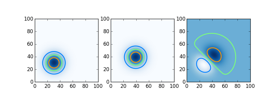
Having seen the parallel computing tools available in each language, we try here a simple distributed computation. Here we try Julia, Chapel, and Python using Dask on a simple distributed-memory stencil problem, two dimensional upwinded advection. A Gaussian blob is advected by a constant velocity field; shown below is the initial condition, the blob moved slightly after a few timesteps, and the difference.

We do this in Julia using DistributedArrays, in Chapel using Stencil-distributed arrays, and in Python using Dask arrays. The relevant code snippets follow below.

@everywhere function get_data_plus_gc(domain, nguard, ngrid)
    if myid() in procs(domain)
        li = localindexes(domain)
        lp = localpart(domain)

        s = size(lp)
        data_plus_gc = zeros(s[1]+2*nguard, s[2]+2*nguard)
        for j in 1:s[2]
            for i in 1:s[1]
                data_plus_gc[i+nguard, j+nguard] = lp[i,j]
            end
        end

        xstart = li[1][1]
        xend   = li[1][end]
        ystart = li[2][1]
        yend   = li[2][end]

        for g in 1:nguard
            xsg = (xstart-1-g + ngrid) % ngrid + 1
            xeg = (xend-1+g) % ngrid + 1

            for j in 1+nguard:s[2]+nguard
                data_plus_gc[nguard+1-g, j] = domain[xsg, j-nguard+ystart-1]
                data_plus_gc[s[1]+nguard+g, j] = domain[xeg, j-nguard+ystart-1]
            end

            #...
        end
    end
    return data_plus_gc
end

@everywhere function advect_data(dens, nguard, ngrid, velx, vely, dx, dy, dt)
    locdens = get_data_plus_gc(dens, nguard, ngrid)

    #...calculate gradients on locdens

    for j in 1+nguard:ny+nguard
        for i in 1+nguard:nx+nguard
            localpart(dens)[i-nguard, j-nguard] -= dt*(velx*gradx[i,j] + vely*grady[i,j])
        end
    end
end

#...

function timestep(dens, nguard, ngrid, velx, vely, dx, dy, dt)
    ps = procs(dens)
    refs = [(@spawnat p advect_data(dens, nguard, ngrid, velx, vely, dx, dy, dt)) for p in ps]
    pmap(fetch, refs)
end

#...

//...

  const ProblemSpace = {1..ngrid, 1..ngrid},
        ProblemDomain : domain(2) dmapped Stencil(boundingBox=ProblemSpace, fluff=(nguard,nguard), periodic=true) = ProblemSpace;

  //...
  var dens: [ProblemDomain] real = 0.0;

  // density a gaussian of width sigma centred on (initialposx, initialposy)
  forall ij in ProblemSpace {
    var x = (ij(1)-1.0)/ngrid;
    var y = (ij(2)-1.0)/ngrid;
    dens(ij) = exp(-((x-initialposx)**2 + (y-initialposy)**2)/(sigma**2));
  }

  for iteration in 1..ntimesteps  {
    // update the boundary conditions - periodic
    dens.updateFluff();

    // calculate the upwinded gradient
    // ...

    dens = dens - dt*(velx*gradx + vely*grady);
//...
}

#...

def dask_step(subdomain, nguard, dx, dy, dt, u):
    """
    map_overlap applies a function to a subdomain of a dask array,
    filling the guardcells in first
    """
    return subdomain.map_overlap(advect, depth=nguard, boundary='periodic',
                                 dx=dx, dy=dy, dt=dt, u=u)


def initial_conditions(x, y, initial_posx=0.3, initial_posy=0.3, sigma=0.15):
    xx, yy = np.meshgrid(x, y)
    density = np.exp(-((xx-initial_posx)**2 + (yy-initial_posy)**2)/(sigma**2))
    return density


if __name__ == "__main__":
    #...

    dens = initial_conditions(x, y)
    subdomain_init = da.from_array(dens, chunks=((npts+1)//2, (npts+1)//2))

    # These create the steps, but they don't actually perform the execution...
    subdomain = dask_step(subdomain_init, 2, dx, dy, dt, u)
    for step in range(1, nsteps):
        subdomain = dask_step(subdomain, 2, dx, dy, dt, u)

    # _this_ performs the execution
    start = time.clock()

As with the stream benchmark, we see that the Julia DistributedArrays require a lot of bookkeeping to use; both Chapel and Dask are much more straightforward.

The one-node timings here aren’t even close. By forcing Chapel to run on each core separately, the performance isn’t that different than Julia. But when informed that there is one “locale” and letting it sort out the details, Chapel benefits dramatically from being able to use multiple levels of parallelism, and with no extra work; on a single 8-processor node, running a 1000x1000 grid with all cores takes the following amount of time:

The 0.4s is not a typo. Threading matters. Admittedly, this is a bit of an extreme case, 1000x1000 isn’t a big grid to distribute over 8 processes, so communications overhead dominates; Julia seems to suffer that overhead even with just one process.

Another interesting thing here is that Python+Numpy+Dask (numba didn’t help here) is competitive even with Chapel if you force Chapel to not use threading on-node, and either made it much easier to write the program than Julia.

Strengths, Weaknesses, and Future Prospects

Both Julia and Chapel are perfectly useable today for problems that fall within their current bailiwicks, at least for advanced users. They are strong projects and interesting technologies. In addition, both have significant potential and “room to grow” beyond their current capabilities; but both face challenges as well.

Julia

Julia’s great flexibility - the metaprogramming and the type system in particular - gives it a very real opportunity to become a platform on which many domanin-specific language are written for particular scientific problems. We see some of that potential in tools like DifferentialEquations.jl, where a simple, general API can nonetheless be used to provide efficient solutions to problems that span a wide range of regimes and structures; the solve() function and the problem definition language essentially becomes a DSL for a wide range of differential equation problems. And Julia’s interactive and dynamic nature makes it a natural for scientists noodling around on problems, performing numerical experiments and looking at the results. While large-scale computing — in an HPC or Spark-style Big-data sense — is not a forte of Julia’s right now, the basic pieces are there and it certainly could be in the future.

Many of Julia’s disadvantages are inevitable flip sides of some of those advantages. Because of the dynamic nature of the language and its reliance on JIT and type inference, it is still not possible to fully compile a Julia script into a static executable, meaning that there will be JIT pauses in initial iterations of running code; too, the dynamic nature of the language relies on garbage collection, which can cause either GC pauses (and thus jitter at scale) or unexpected memory pressure throughout execution. Similarly, the fact that it’s so easy to contribute a package to the Julia package ecosystem means that the package listing is littered with abandoned and broken packages.

But some of the disadvantages seem more self-inflicted. While the language has been public and actively developed for over five years, the language is still at v0.6. While any language will evolve over time, the Julia community has spent the past five years contininually re-litigating minor but foundational decisions of syntax and behaviour in the interests of conceptual purity – v0.4 in late 2015 changed the capitalization of unsigned integer types and radically changed the dictionary syntax, while 0.5 in late 2016 dramatically (although less dramatically than originally proposed after community pushback) changed the behaviour of arrays (!!) in an event termed the Arraypocolypse. Discussions on the correct choice for string concatenation operator span enormous and non-stop github issue discussions from late 2012 to mid 2015. At least one more round of significant breaking changes are planned before a 1.0 release. As a result, most non-trivial example code online simply doesn’t work; thus also the accelerated bitrot of software in the Julia package listing. It has been difficult to implement new functionality on top of base Julia; it’s hard to build powerful parallel computing tools when one can’t even depend on the behavour of arrays. I would have liked to use Intel’s ParallelAccelerator for Julia to see how it worked on the advection problem above, for instance, but Julia 0.6 breaks the ParallelAccelerator, and Julia 0.6 is needed for the @simd feature with DistributedArrays.

So Julia living up to its potential is not a given. If I were on Julia’s project team, things that would concern me would include:

Peak Julia?

Julia grew very quickly early on, but since then seems to have topped out; for example, flat google trends interest, and falling off the radar of “languages to watch” lists such as the Redmonk language rankings, This may be unfair; these trends may say more about the large initial surge of interest than stagnation or decline. “A hugely popular scientific programing language” almost seems like an oxymoron, after all. Declining Stack Overflow interest may simply reflect that the community has successfully moved discussion to its discourse site. A five-year old language for numerical computing that still hasn’t reached 1.0 but has popularity comparable to Rust (which started at the same time but is a more general systems-programming language) or Fortran (which has an enormous installed base) is pretty remarkable; further growth may inevitably be more modest simply because of the small number of scientific programmers out there. Still, I think one would want to see interest growing ahead of a 1.0 release, rather than flat or declining.

Instability driving off users, developers

Very early on, community members who used Julia started building what became JuliaStats, with R-like data frames, data tables, random distributions, and a growing number of statistics and machine-learning tools built atop. This took significant developer effort, as fundamental to statistical use cases is “Not Available” or “NA” values, with semantics different from the NaNs that we in the simulation computing community are so frequently (if usually unintentionally) familar with. Thus dataframes and tables couldn’t simply be built directly on top of numerical arrays of basic numerical types, but took some effort to build efficient “nullable” types atop of. But partly because of instability in the underlying language, Julia DataFrames and DataArrays have themselves been under flux, which is show-stopping to R users considering Julia, and demoralizing to developers. Many other similar examples exist in other domains. If it is true that there is declining or stagnant interest in Julia, this would certainly be a contributing factor.

The JIT often needs help, even for basic numerical computing tasks

Julia is designed around its JIT compiler, which enables some of the language’s very cool features - the metaprogramming, the dynamic nature of the language, the interactivity. But the JIT compiler often needs a lot of help to get reasonable performance, such as use of the the @inbounds macro in the stencil calculation. Writing numerical operations in the more readable vectorized form (like for the stream example in Chapel, C = A + B rather than looping over the indices) has long been slow in Julia, although a new feature may have fixed that. A third party package exists which helps many of the common cases (speeding up stencil operations on rectangular arrays), which on one hand indicates the power of Julia metaprogramming capabilities. But on the other, one might naturally think that fast numerical operations on arrays would be something that the core language came with. Part of the problem here is that while the Julia ecosystem broadly has a very large number of contributors, the core language internals (like the JIT itself) has only a handful, and complex issues like performance problems can take a very long time to get solved.

The 800lb pythonic gorilla

Python is enormously popular in scientific and data-science type applications, has huge installed base and number of packages, and with numpy and numba can be quite fast. The scientific computing community is now grudgingly starting to move to Python 3, and with Python 3.5+ supporting type annotations, I think there’d start to be a quite real concern that Python would get Julia-fast (or close enough) before Julia got Python-big. The fact that some of Julia’s nicest features like notebook support and coolest new projects like Dagger rely on or are ports of work originally done for Python (ipython notebook and Dask) indicate the danger if Python gets fast enough.

Of those four, only the middle two are completely under the Julia team’s control; a v1.0 released soon, and with solemn oaths sworn to have no more significant breaking changes until v2.0 would help developers and users, and onboarding more people into core internals development would help the underlying technology.

Chapel

If I were on the Chapel team, my concerns would be different:

Adoption

It’s hard to escape the fact that Chapel’s user base is very small. The good news is that Chapel’s niche, unlike Julia’s, has no serious immediate competitor — I’d consider other productive parallel scientific programming languages to be more research projects than products — which gives it a bit more runway. But the niche itself is small, and Chapel’s modest adoption rate within that niche needs to be addressed in the near future if the language is to thrive. The Chapel team is doing many of the right things — the package is easy to install (no small feat for a performant parallel programming language); the compiler is getting faster and producing faster code; there’s lots of examples, tutorials and documentation available; and the community is extremely friendly and welcoming — but it seems clear that users need to be given more reason to start trying the language.

Small number of external contributors

Admittedly, this is related to the fact that the number of users is small, but it’s also the case that contributing code is nontrivial if you want to contribute it to the main project, and there’s no central place where other people could look for your work if you wanted to have it as an external package. A package manager would be a real help, and it doesn’t have to be elaborate (especially in the initial version).

Not enough packages

In turn, this is caused by the small number of external contributors, and helps keep the adoption low. Chapel already has the fundamentals to start building some really nice higher-level packages and solvers that would make it easy to start writing some types of scientific codes. A distributed-memory n-dimensional FFT over one of its domains; the beginnings of a Chapel-native set of solvers from Scalapack or PETSc (both of which are notoriously hard to get started with, and in PETSc’s case, even install); simple static-sized R-style dataframes with some analysis routines; these are tools which would make it very easy to get started writing some non-trivial scientific software in Chapel.

Too few domain maps and layouts

Being able to, in a few lines of code, write performant, threaded, NUMA-aware, and distributed memory operations on statically-decomposed rectangular multidimensional arrays, and have that code work on a cluster or your desktop is amazing. But many scientific problems do not match neatly onto these domains. Many require dynamically-sized domains (block-adaptive meshes) or load balancing (tree codes, dynamic hash tables); others may be static but not quite look like CSR-sparse arrays. Domain maps, layouts, and the parallel iterators which loop over them are the “secret sauce” of Chapel, and can be written in user code if the underlying capabilities they need are supported, so they can be contributed externally, but there is little documention/examples (compared to that on using existing domain maps) available.

The good news is that these items are all under the Chapel community’s control. Programs that are natural to write in Chapel currently are easy to write and can perform quite well; the goal then is to expand the space of those programs by leveraging early adopters into writing packages.

My conclusions

This is entitled “My conclusions” because my takeaways might reasonably be different than yours. Here’s my take.

Both projects are strong and useable, right now, at different things

I’d have no qualms about recommending Chapel to someone who wanted to tackle computations on large distributed rectangular arrays, dense or sparse, or Julia for someone who had a short-lived project and wanted something interactive and requiring only single-node or coordinator-worker computations (or patterns that were more about concurrency than parallelism). Julia also seems like a good choice for prototyping a DSL for specific scientific problems.

Neither project is really a competitor for the other; for Julia the nearest competitor is likely the Python ecosystem, and for Chapel it would be status quo (X + MPI + OpenMP/OpenACC) or that people might try investigating a research project or start playing with Spark (which is good at a lot of things, but not really scientific simulation work.)

Scientific computing communities are very wary of new technologies (it took 10+ years for Python to start getting any traction), with the usual, self-fulfulling, fear being “what if it goes away”. I don’t think there’s any concern about dead code here for projects that are started with either. Chapel will be actively supported for another couple of years at least, and the underlying tools (like GASNet) underpin many projects and aren’t going anywhere. One’s code wouldn’t be “locked into” Chapel at any rate, as there are MPI bindings, so that there’s always a path to incrementally port your code back to MPI if you chose to. For Julia, the immediate worry is less about lack of support and more that the project might be too actively maintained; that one would have to continually exert effort to catch your code up with the current version. In either case, there are clear paths to follow (porting or upgrading) to keep your code working.

Both projects have as-yet untapped potential

What’s exciting about both of these projects is how far they could go. Chapel already makes certain class of MPI+OpenMP type programs extremely simple to write with fairly good performance; if that class of programs expands (either through packages built atop of current functionality, or expanded functionality through additional well-supported domain maps) and as performance continues to improve, it could make large-scale scientific computation accessible to a much broader community of scientists (and thus science).

Julia has the same potential to broaden computational science on the desktop, and (at least in the near term) for computations requiring only minimal communication like coordinator-worker computations. But Python is already doing this, and making suprising inroads on the distributed-memory computing front, and there will be something of a race to see which gets there first.