ARLS, Automatically Regularized Least Squares

(I have a guest blogger today. Ron Jones worked with me in 1985 for his Ph. D. from the University of New Mexico. He retired recently after nearly 40 years at Sandia National Labs in Albuquerque and now has a chance to return to the problem he studied in his thesis. -- CBM)

by Rondall Jones, rejones7@msn.com

Our interest is in automatically solving difficult linear systems,

  A*x = b

Such systems often arise, for example, in "inverse problems" in which the analyst is trying to reverse the effects of natural smoothing processes such as heat dissipation, optical blurring, or indirect sensing. These problems exhibit "ill-conditioning", which means that the solution results are overly sensitive to insignificant changes to the observations, which are given in the right-hand-side vector, b .

Here is a graphic showing this behavior using a common test matrix, a 31 x 31 Hilbert matrix, with the blue line being the ideal solution that one would hope a solver could compute. The jagged red line shows the result of a traditional solver on this problem.

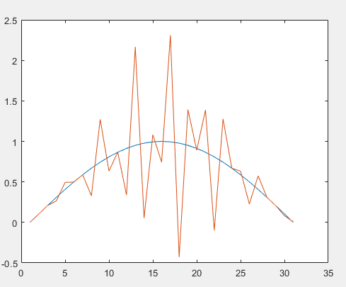
In fact this graph is extremely mild: the magnitude of the oscillations often measure in the millions, not just a little larger than the true solution. Traditionally analysts have approached this issue in the linear algebraic system context by appending equations to A*x = b that request each solution value, x(i), to be zero. Then, one weights these conditioning equations using a parameter usually called "lambda". We will call it p here. What we have to solve then is this expanded linear system:

   [ A ; p*I] * x = [b; 0]

If we decompose A into its Singular Value Decomposition

   A = U * S * V'

and multiply both sides by the transpose of the augmented LHS, the resulting solution to is

   x = V * inv(S^2 + p^2*I) * S * U' * b

instead of the usual

   x = V * inv(S) * U' * b

It is convenient in the following discussion to represent this as

   x = V * PCV

where

   PCV = inv(S) * U' * b

is what we call the Picard Condition Vector. Then x is computed in the usual SVD manner with the change that each singular value S(i) is replaced by

   S(i) + p^2/S(i)

This process is called Tikhonov regularization.

Using Tikhonov regularization successfully requires somehow picking an appropriate value for p. Cleve Moler has for many years jokingly used the term "eyeball norm" to describe how to pick p. "Try various values of p and pick the resulting solution (or its graph) that 'looks good'".

My early work in attempting to determine lambda automatically was based instead on determining when the PCV begins to seriously diverge. Beyond that point one can be fairly sure that noise in b is causing U'*b to decrease more slowly than inv(S) is increasing, so their product, which is the PCV, starts growing unacceptably. Such an algorithm can be made to work and versions of my work have been available in various forms over the years. But determining where the PCV starts growing unacceptably (which I refer to as the usable rank) is based on heuristics, moving averages, and such, as of which require choices of moving average lengths and other such parameters. This is not an optimal situation, so a I began trying to redesign algorithms that do not use any heuristics.

How do we do that algorithmically? Per Christian Hansen gave a clue to this question when he said (my re-phrasing) that "the analyst should not expect a good solution for such a problem unless the PCV is 'declining'". We note that this adage is a context-specific application of a general requirement that when a function is represented by an orthogonal expansion the coefficients of the orthogonal basis functions should eventually decline toward zero. If this behavior does not happen, then typically either the model is incomplete or the data is contaminated. In our case the orthogonal basis is simply the columns of V, and b is the set of coefficients that would be expected to decline. A good working definition of "declining" has been hard to nail down. The algorithm in ARLS has implemented this concept using two specific essential steps:

So, Phase 1 of ARLS searches a large range of values of p (remember, p is Tikhonov's "lambda") to find a value just barely large enough to make the slope of the parabolic fit entirely negative or zero. This gives us a tight lower bound for the "correct" value of p.

Phase 2 of ARLS is much simpler. Since p is the minimum usable regularization parameter, the solution tends to be less smooth and less close to the ideal solution than optimum. So we simply increase p slightly to let the shape of the graph of x smooth out. Our current implementation increases p until the residual (that is, norm(A*x-b)) of the solution increases by a factor of 2. This is, unfortunately, a heuristic. But an appropriate value of it can be determined by “tuning” the algorithm on a wide range of test problems.

We call this new algorithm Logarithmic Picard Condition Analysis. (If the problems you work on seem to need a bit more relaxation you can, of course, increase the number 2 a bit. It is 5 lines from the bottom of the file.) In the example shown in the graphic above, ARLS produces the blue line so closely that the ideal solution and ARLS computed solution are indistinguishable.

In addition to ARLS(A,b) itself, we provide two constrained solvers built on ARLS which are called just like ARLS:

Try ARLS. It's available from the MATLAB Central File Exchange, #130259, at this link.

Get the MATLAB code

Published with MATLAB® R2023a