Matrices In Action, Grafix 2.0

The 4-by-4 matrices in the panels on the following screenshots are at the heart of computer graphics. They describe objects moving in three-dimensional space and are essential to MATLAB's Handle Graphics, to CAD (Computer Added Design) packages, to CGI (Computer Graphics Imagery) in films, and to most popular video games.

Contents

Grafix 2.0

Here is the opening screen from version 2.0 of Grafix, my tool for investigating the matrices involved in 3-D computer graphics. The MATLAB code for Grafix is availble here.

I am interested in the matrix in the panel, which I call M. Many matrices like this one describe the dyamic transformations to be made on a set of target objects in a complex three-dimensional scene. This particular M is the product of a scaling and a rotation that results in the size and orientation of the plane shown.

I also want to point out the coordinate axes being used. This is view(3), MATLAB's default 3-D cordinate system. The positive $x$-axis goes up and to the right on the screen, the positive $y$-axis up and to the left, and the positive $z$-axis goes straight up.

Rotations

The homogeneous coordinates system used in modern computer graphics makes it possible to describe rotations, translations and many other operations with 4-by-4 matrices. These matrices operate on vectors with the position of an object in the first three components and, for now, a one as the fourth component, eg. [ $x$, $y$, $z$, 1 ]',

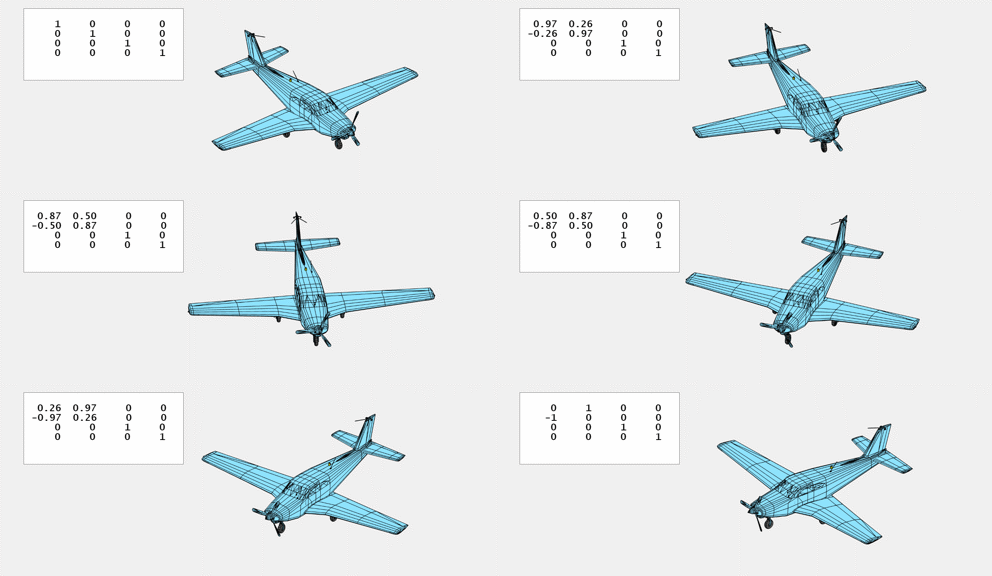
Rotations are described by products of these matrices, each of which operates on only two of the first three components of the vector. The first matrix, $R_x$, leaves $x$ unchanged while it rotates $y$ and $z$. The second matrix, $R_y$, leaves $y$ unchanged while it rotates $x$ and $z$. And the third matrix, $R_z$, leaves $z$ unchanged while it rotates $x$ and $y$.

$$ R_x(\theta) = \left[ \begin{array}{rrrr} 1 & 0 & 0 & 0 \\ 0 & \cos{\theta} & -\sin{\theta} & 0 \\ 0 & \sin{\theta} & \cos{\theta} & 0 \\ 0 & 0 & 0 & 1 \end{array} \right] $$

$$ R_y(\theta) = \left[ \begin{array}{rrrr} \cos{\theta} & 0 & -\sin{\theta} & 0 \\ 0 & 1 & 0 & 0 \\ \sin{\theta} & 0 & \cos{\theta} & 0 \\ 0 & 0 & 0 & 1 \end{array} \right] $$

$$ R_z(\theta) = \left[ \begin{array}{rrrr} \cos{\theta} & -\sin{\theta} & 0 & 0 \\ \sin{\theta} & \cos{\theta} & 0 & 0 \\ 0 & 0 & 1 & 0 \\ 0 & 0 & 0 & 1 \end{array} \right] $$

Pitch, Roll, and Yaw

The terms pitch, roll and yaw are often used to describe the motion of vehicles like aircraft, marine craft, and spacecraft. Pitch is $R_x$, rotation about the $x$-axis.

Roll is $R_y$, rotation about the $y$-axis.

And yaw is $R_z$, rotation about the $z$-axis.

Translations

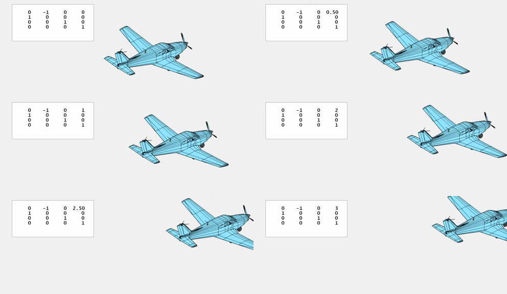
Translations are described by matrices with values in the fourth column. Multiplying a vector by one of these matrices produces a translation in the direction of the corresponding axis.

$$ T_x(\delta) = \left[ \begin{array}{rrrr} 1 & 0 & 0 & \delta \\ 0 & 1 & 0 & 0 \\ 0 & 0 & 1 & 0 \\ 0 & 0 & 0 & 1 \end{array} \right] $$

$$ T_y(\delta) = \left[ \begin{array}{rrrr} 1 & 0 & 0 & 0 \\ 0 & 1 & 0 & \delta \\ 0 & 0 & 1 & 0 \\ 0 & 0 & 0 & 1 \end{array} \right] $$

$$ T_z(\delta) = \left[ \begin{array}{rrrr} 1 & 0 & 0 & 0 \\ 0 & 1 & 0 & 0 \\ 0 & 0 & 1 & \delta \\ 0 & 0 & 0 & 1 \end{array} \right] $$

While it is true that translations could be accomplished simply by adding the increment to the specified coordiate, the use of matrix multiplication allows translations to be combined in a uniform way with rotations and other operations. The arithmetic units on today's Graphics Processing Units, GPUs, are designed to do 4-by-4 matrix multiplications at speeds hundreds of times faster than general purpose Central Processing Units, CPUs.

Horizontal and Vertical

Inspired by David Singmaster's notation for Rubik's cubes, L, R, B, F, U, and D, we can use the descriptive terms left and right for horizontal motion in the $x$ direction; back and forth for horizontal motion in the $y$ direction; and up and down for vertical motion in the $z$ direction.

$T_x$, left and right.

$T_y$, back and forth.

$T_z$, up and down.

Scalings

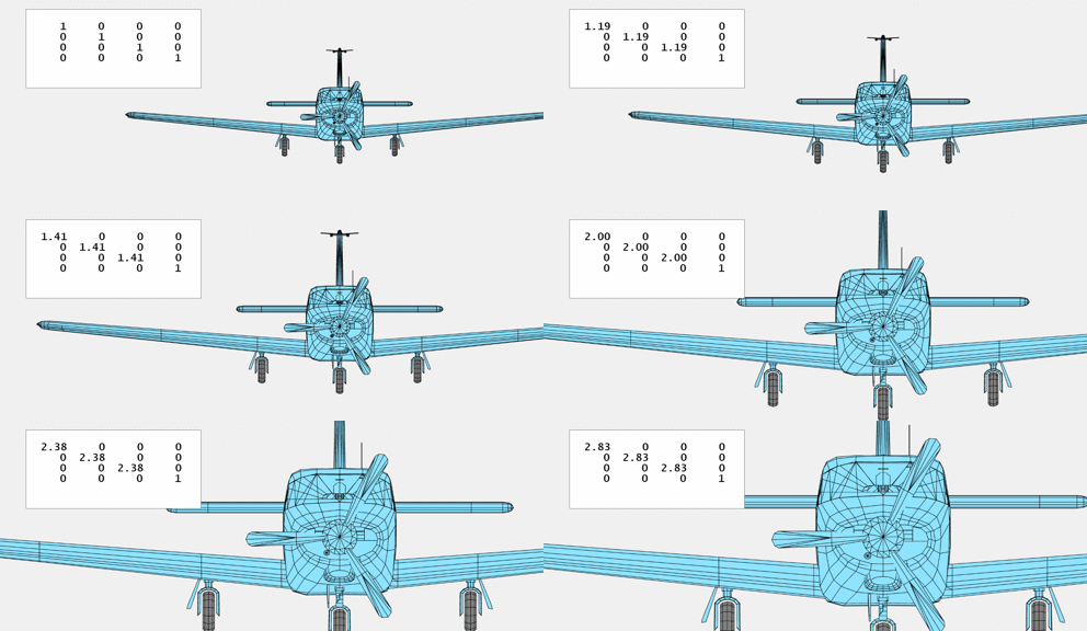
This matrix applies a single scaling factor to all three axes.

$$ S(\sigma) = \left[ \begin{array}{rrrr} \sigma & 0 & 0 & 0 \\ 0 & \sigma & 0 & 0 \\ 0 & 0 & \sigma & 0 \\ 0 & 0 & 0 & 1 \end{array} \right] $$

Larger and Smaller

$S$

Suggestions

Refresh your browser to syncronize the animations.

Download your own self-archiving copies of

Get the MATLAB code

Published with MATLAB® R2023a