R-squared. Is Bigger Better? - hpc.social - Aggregated Commercial Blog

The coefficient of determination, R-squared or R^2, is a popular statistic that describes how well a regression model fits data. It measures the proportion of variation in data that is predicted by a model. However, that is all that R^2 measures. It is not appropriate for any other use. For example, it does not support extrapolation beyond the domain of the data. It does not suggest that one model is preferable to another.

I recently watched high school students participate in the final round of a national mathematical modeling competition. The teams' presentations were excellent; they were well-prepared, mathematically sophisticated, and informative. Unfortunately, many of the presentations abused R^2. It was used to compare different fits, to justify extrapolation, and to recommend public policy.

This was not the first time that I have seen abuses of R^2. As educators and authors of mathematical software, we must do more to expose its limitations. There are dozens of pages and videos on the web describing R^2, but few of them warn about possible misuse.

R^2 is easily computed. If y is a vector of observations, f is a fit to the data and ybar = mean(y), then

   R^2 = 1 - norm(y-f)^2/norm(y-ybar)^2

If the data are centered, then ybar = 0 and R^2 is between zero and one.

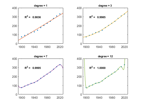
One of my favorite examples is the United States Census. Here is the population, in millions, every ten years since 1900.

   t         p
  ____    _______
  1900     75.995
  1910     91.972
  1920    105.711
  1930    123.203
  1940    131.669
  1950    150.697
  1960    179.323
  1970    203.212
  1980    226.505
  1990    249.633
  2000    281.422
  2010    308.746
  2020    331.449

There are 13 observations. So, we can do a least-squares fit by a polynomial of any degree less than 12 and can interpolate by a polynomial of degree 12. Here are four such fits and the corresponding R^2 values. As the degree increases, so does R^2. Interpolation fits the data exactly and earns a perfect core.

Which fit would you choose to predict the population in 2030, or even to estimate the population between census years?

R2_census

Thanks to Peter Perkins and Tom Lane for help with this post.

Get the MATLAB code

Published with MATLAB® R2024a