Two Flavors of SVD

MATLAB has two different ways to compute singular values. The easiest is to compute the singular values without the singular vectors. Use svd with one output argument, s1.

  s1 = svd(A)

The alternative is to use svd with three outputs. Ignore the first and third output and specify the second output to be a column vector, s2.

  [~,s2,~] = svd(A,'vector')

The MathWorks technical support team receives calls from observant users who notice that the two approaches might produce different singular values. Which is more accurate, s1 or s2? Which is faster? Which should we use?

I found myself asking the same questions.

A key feature of all our experiments is the rank of the matrix. Let's investigate three cases: a rank 2 matrix, a low rank matrix, and a full rank matrix.

Checkerboard

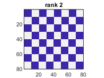
The first example, motivated by a recent query, is an 80-by-80 matrix of zeros and ones derived from the checkerboard function in the Image Processing Toolbox.

    A = double(checkerboard > 0);

The rank of the checkerboard matrix is 2.

    r = rank(A)

r =
     2

The image function provides the same portrait of A as its spy plot.

    imagem(A)
    title('rank 2')

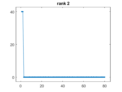
Let's begin with the exact singular values. The two nonzero singular values are both equal to 40. The zero singular value has multiplicity 78.

    s = [40; 40; zeros(78,1)];
    disp('  s =')
    disp(s(1:5))
    disp('     :')
    disp(s(end-2:end))

A perfect plot of the singular values of a rank 2 matrix would look like this.

    plotem(s)
    title('rank 2')

What do we get when we actually compute the SVD of the checkerboard?

The built-in SVD function uses Householder reflections to reduce the matrix to bidiagonal form. When the vectors are not required, a divide and conquer iteration then reduces the bidiagonal to diagonal. In all our examples, after divide and conquer has found the nonzero singular values, all that remains is roundoff error. Despite this fact, the iterations are continued in order to find all singular values "to high relative error independent of their magnitudes." We have roundoff in roundoff, then roundoff in roundoff in roundoff, and so on.

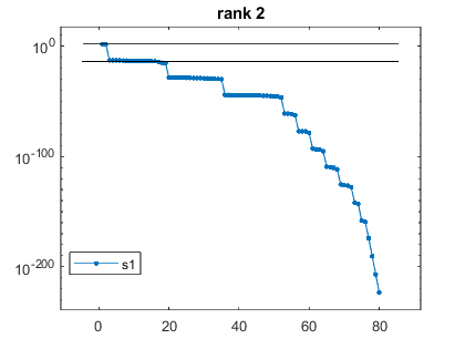
The following logarithmic plot of s1 for the checkerboard matrix shows the phenomenon that I like to call "cascading roundoff". There are lines at norm(A) and at

    tol = eps(norm(A))

tol =
   7.1054e-15

This is the tolerance initially involved in the convergence test. The steps in the plot are at powers of tol.

    s1 = svd(A);
    plotem(s1,inf)
    title('rank 2')

If we specify three outputs, the iterative portion of the SVD function uses a traditional QR iteration with a more conservative convergence criterion instead of divide and conquer. There is no cascading roundoff. All the s2 singular values that would be zero with exact computation are of size tol.

    [~,s2,~] = svd(A,'vector');
    plotem(s1,s2,[-48,4])
    title('rank 2')

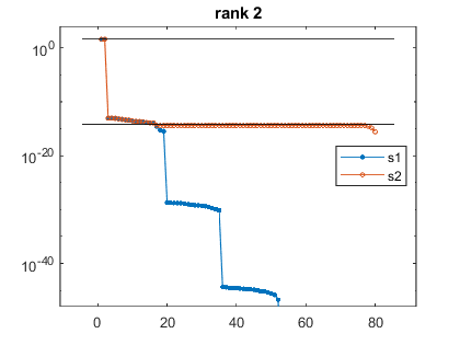
The plots of s1 and s2 are very different, and neither plot looks like the plot of the exact answer. However, all three plots agree about the double value at 40. And all the disagreements, including the cascading roundoff in s1, are below the line at tol.

The checkerboard example shows that s1 and s2 can be very different, but s1 and s2 are much closer to each other than either is to the right answer.

Low Rank

For a matrix with rank between 2 and full order n, we can use the venerable Hilbert matrix. We have a row vector j and a column vector k in a singleton expansion.

    n = 80;
    j = 1:n;
    k = (1:n)';
    A = 1./(k+j-1);

The effective rank turns out to be 17.

    r = rank(A)

r =
    17

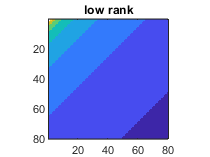
The elements of this Hilbert matrix vary over three orders of magnitude, so a logarithmic image is appropriate.

    imagem(floor(log2(A)))
    title('low rank')

Compare the one-output and the three-output singular values,

    s1 = svd(A);
    [~,s2,~] = svd(A,'vector');
    plotem(s1,s2,[-22,3])
    title('low rank')

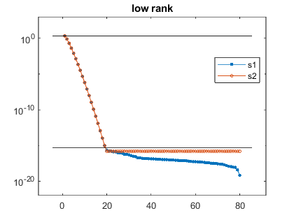
The results s1 and s2 agree about the first 17 values and all disagreements are below the line at tol.

Full Rank

Using the same column vector k and row vector j in another example of single expansion produces a full rank matrix.

    A = min(k,j);

Check that A has full rank.

    r = rank(A)

r =
    80

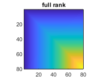
The logarithm is not needed for this image.

    imagem(A)
    title('full rank')

Compare the one-output and the three-output singular values,

    s1 = svd(A);
    [~,s2,~] = svd(A,'vector');
    plotem(s1,s2,[-2,4])
    title('full rank')

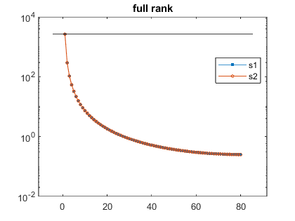
With full rank, all values of s1 and s2 are essentially equal. Any line at tol would be irrelevant.

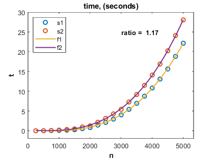
Timing

Which is faster, s1 or s2?

One extensive timing experiment involves matrices with full rank and with orders

   n = 250:250:5000

The times measured for computing s1 and s2 are shown by the o's in the following plot.

Since the time complexity for computing SVD is O(n^3), we fit the data by cubic polynomials. For large n, the time required is dominated by the n^3 terms. The ratio of the coefficients of these dominate terms is

   ratio = 1.17

In other words, for large problems s1 is about 17 percent faster than s2.

    timefit

Remarks

I will admit to a personal preference for s2 over s1. I am more familiar with QR than I am with divide and conquer. As a result, I have more confidence in s2.

I realize that the LAPACK divide and conquer driver DSVDD can achieve the stated goal of finding all singular values "to high relative error independent of their magnitudes" if the input A is bidiagonal and known exactly. But I don't see that in MATLAB with s1. I suspect that MATLAB does not make a special case for bidiagonal svd.

I will be very happy to see any other examples. Please comment.

Software

This blog post is executable. You can publish it if you also have the three files in Checkerboard_mzip.

Get the MATLAB code

Published with MATLAB® R2024b

hpc.social

Contents